
What follows are some interesting (to me, anyway!) examples of math applications, numerical calculations and their interpretations. I used ALAMA Calculator for the calculations, but of course, any capable math software or hardware could be used in place of it. If you’re a math programmer, you might find it an entertaining exercise to develop you own solutions on your platform of choice (Matlab, octave, R, Maple, Mathematica, etc) for these examples — or, for that matter, write your own ALAMA Calculator programs instead of using mine. In case you want to play with some of the examples I present below, all of the ALAMA programs that I use in the topics below are included in zipped folder FunWithALAMA listed below. Most of these programs require version (1.1.2) of ALAMA to work, so if there is a version for your platform, you should download it first. Many of these examples involve a discussion with enough math discussion and formulation that I found it very difficult to present them in plain text format, so in those cases I attached pdf files that give full presentations.
The list of Fun withs has become so lengthy (and still growing) that I decided to give a Table of Contents of a sort with very brief descriptions of the topics. Here it is:
Fun with Polygons: Every closed polygon, even self-intersecting ones, can be gradually smoothed out to form an approximate ellipse. A lovely blend of matrix theory and computation!
Fun with Number Theory: Did you know that there is some integer power of 2 whose first nine digits are exactly your SSN, whatever it is? Nope, I didn’t either, but it’s true and here is an analysis of that fact along with the basic number theory required (an introduction, really).
Fun with Coding: Gives a cautionary tale involving an uncritical assumption of standard complexity theory result and illustrates the importance of reading the fine print.
Fun with RREF: Examines two interesting but lesser known matrix factorizations, CR and CWB, that derive from the reduced row echelon form (RREF) of a matrix.
Fun with Probability: Application of Bayes’ Theorem from probability theory can draw some surprisingly unintuitive conclusions to some very practical problems.
Fun with Infinity. A very non-technical discussion on why the set of real numbers is “uncountable” and explanation of what that means for non-specialists.
Fun with Sudoku: Not a whole lot of math here, just Sudoku fun and a simple program that will handle Easy and Very Easy cases, plus give you a start on the harder ones.
Fun with Performance: Say what? Well, this is about performance of quantities that change over time — like an investment fund. See this article for examples, including a political one.
Fun with Your IRA: Huh? That’s fun?? Well, another matter of opinion. But suppose you’re about to start your RMD withdrawals, don’t think it’s likely you’ll make it past 85 and want to see how much of your IRA might remain for your kids? See this section for possible answers.
All of the ALAMA programs used in these discussions are contained in the following zipped folder for download:
Fun with Polygons: Recently, I ran across an incredibly charming example of how theory, application and computation blend together beautifully in linear algebra. The example is the subject of the SIAM 2018 John von Neumann Lecture delivered by an outstanding researcher of numerical linear algebra, Charles Van Loan, where he made some fascinating observations on how to systematically “untangle” a randomly selected polygon, no matter how convoluted it is. The idea is as follows: Say that the polygon is described by distinct vertices (x0, y0),…,(xn, yn), where the last vertex is connected to the first. Consider this iterative process for constructing successive polygons:
- Construct the initial polygon by a random selection of x- and y-coordinates for n+1 vertices, (x0,y0),…,(xn, yn).
- Translate the polygon so that the centroid of the resulting polygon is at the origin (obtained by averaging each of the sums of x- and y-coordinates, dividing by n+1 and subtracting the results from each coordinate).
- Use the vector 2-norm to normalize the size of the polygon so that the norms of the vectors of x- and y-coordinates coordinates are both one.
- Plot this polygon in the xy-plane.
- Construct a new polygon from the old by replacing each vertex (xi, yi ) by the midpoint vertex ((xi, yi) + (xi+1, yi+1))/2 of the segment connecting these two points of the polygon, where the indices are computed mod n+1.
- Repeat steps 3-5 until the polygon shapes settle down to an approximately constant form.
The tools in this exploration are two ALAMA calculator programs (VanLoanExampleN.alm and VanLoanExampleNcplx.alm) which are available in the in the folder ALAMAprograms and the above file FunWithALAMA.zip or you may write your own programs that achieve the same results. The suffix ’N’ means that the standard normal distribution was used to generate it. In addition, the suffix “cplx” means that the following alternative method was used in place of steps 3 and 4: View the x- and y-coordinates of a point as coordinates of the complex number z = x + yi, normalize the resulting vector of complex numbers with the complex 2-norm, plot the resulting polygon in the complex plane and construct a new polygon by averaging successive vertices. Here are pictures of the results where the number of vertices is 14 and 10 iterations of the process above are used to generate each figure using the real and complex versions of the algorithm. The figures are scaled up by factors of 3 and 4, resp., and colors for successive figures starting with the random polygon are black, red, green, blue, dark yellow and cyan:

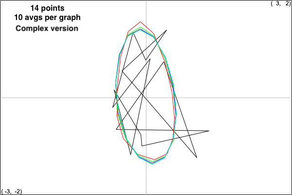
Every time you repeat this experiment, you get similar results: The limiting polygon takes a familiar shape. How to explain this settling down to a constant convex figure? Linear algebra to the rescue, and I’ll leave the full explanation for the reader to explore, but here’s the first step: the averaging of step 5 can be viewed as a matrix/vector multiplication, where the vectors are vectors of x- and y- coordinates (or a single vector with complex coordinates x + yi in the case of the complex version).
Fun with Number Theory: I’m a fan of Great Courses offerings and recently I had the pleasure of watching the offering “Introduction to Number Theory” by Professor Edward Burger. The course was designed for those who may have been long away from their high school algebra (as it should have been), so it wasn’t terribly exciting for me personally until he made this delightful “come-on” in Lecture 2: You are assured that there is some power of 2 whose first nine digits are exactly your social security number. I had to wait till Lecture 21 to begin to see some justifications for this “powers of 2” assertion. I was intrigued by some unproved statements concerning this claim, so I went about writing my own proofs in the spirit of Professor Burger’s course: requiring no more than high school algebra and geometry. In fact, I ended up writing a brief essay, which includes a concise introduction to number theory complete with a few exercises. You can see it in the following pdf file, which you may have to download if your viewer doesn’t show it.
ALAMA Calculator helped me in two ways: First, experimentation with it gave me the clues that I needed to write proofs of the necessary results substantiating the “powers of 2” claim. Secondly, I had a bit of fun verifying simpler versions of the claim which are included as exercises at the end of “Fun with Numbers”. If you want to play around with these ideas there are a few ALAMA Calculator programs that you might find helpful, namely a sorting program, programs to construct/deconstruct continued fractions and just for fun, a gcd program. Another program that I found useful in my experimentation was InsertionSortCndx.alm. This program sorts a list of numerical data, but also preserves the initial indices of the sorted items, so that the initial positions of each sorted item held before sorting are known. These are contained in the folder ALAMAprograms and the zipped folder FunWithALAMA.zip.
Fun with Coding: Speaking of “sorting”, some standard topics in an introductory computer science course are algorithms and their complexity. The problem of sorting a list of numbers (or words or anything else that can be linearly ordered) can be used to illustrate these ideas. In fact, I needed a sorting program to help me find proofs of certain theorems in the “FunWithNumberTheory” pdf. I have claimed that ALAMA Calculator is fully programmable, so I decided to put my feet to the fire and write suitable sorting programs on it. To add to the challenge, I decided that the programs should only use the single variable C that consists of the list of numbers to be sorted as a row vector augmented by two entries that are the start and finish of the section of C to be sorted. One reason for this constraint is that ALAMA Calculator only has 10 named variables, so in case others are already in use, one should try to use as few extra variables as possible.
So, what algorithms to use? I decided to try two well known methods: insertion sort and quicksort, which resulted in the ALAMA programs InsertionSortC.alm and QuickSortC.alm. (Aside to programmers: Along the way I realized that it was very helpful to expand the functionality of the Rpt() command, which I did in version (1.1.1).) Given that n items are to be sorted, the insertion sort algorithm is known to have best, average and worst case complexities of O(n), O(n^2) and O(n^2), respectively. For quicksort, the corresponding complexities are O(n log(n)), O(n log(n)) and O(n^2). Accordingly, one is tempted to always use quicksort instead of insertion sort. On average, this is ok, but it’s instructive to experiment with different lists of items and compare the timings for each method. Try this experiment on ALAMA Calculator:
B = [RndN([1:400]), 1, 400];
C = B;
Now load the program InsertionSortC.alm and execute the command Rpt(1,1), but also use a timer to determine time of execution. Next, set C equal to B again (to insure that we’re comparing sorting of the same list) and repeat this experiment with the program QuickSortC.alm. My timing results on my mac were about 22 second for insertion sort and about 3 seconds for quicksort. This is what you’d expect, right? Next, repeat the whole experiment with these initial values: B = [Ones(1,400), 1, 400]; C = B; My timing results were surprising: about 6 seconds for insertion sort and 25 seconds for quicksort. Say what? One learns in a detailed study of these algorithms that quicksort has more of a problem with many equal items in the list. Moral: Matters are a bit more nuanced than one might expect, so one shouldn’t depend only on the stated average complexities of these algorithms.
Fun with RREF: So what is “RREF”? It’s the acronym for “reduced row echelon form”, so you’ll need some exposure matrix analysis in order to appreciate this discussion. Recently, I ran across a charming article by Gilbert Strang and Cleve Moler titled “LU and CR elimination” which appeared in the March 2022 edition of the journal SIAM Review. It’s about two matrix factorizations that, even as an author of a linear algebra text (ALAMA), I had not seen before. Here they are, but first a concrete example to fix ideas:

OK, so what? Well, first notice the structure of C: It consist of the three columns of A in the first, third and fourth positions, which is exactly where the pivot elements of RREF occur, which yields the three columns of the 3×3 identity. In other words, these are the three independent columns of A and the other two columns are linear combinations of these with coefficients peering at us from the corresponding columns of the RREF. See it? Well, check that for A, column 2 is just 1*(column 1) and column 5 is just -2*(column 1)+3*(column 3)-1*(column 4), just as the columns 2 and 5 in R tell us. Next notice that R is just the RREF of A with the bottom zero rows deleted (‘reduced RREF’, ya think?).
The programs CR.alm, CWB.alm and TestA.alm are all contained in the FunWithALAMA zipped folder. Now for the fun part: If you’re using ALAMA calculator, use the editor to construct the 4×5 matrix A (or simply load TestA.alm), then open the file CR.alm, execute Rpt(1,1)<Enter>, followed by C<Enter>, then U<Enter>, then C*U<Enter>. The output:
“Compute CR decomposition for matrix A. Variables used are C, U, P, u, v, with the C matrix as C, R matrix as U. First construct matrix A, then load and execute with ‘Rpt(1,1)’. “
Out>C :
1, 2, 1 ;
2, 4, -2 ;
3, 2, -4 ;
3, 6, -1
Out>U :
1, 1, 0, 0, -2 ;
0, 0, 1, 0, 3 ;
0, 0, 0, 1, -1
Out>C * U :
1, 1, 2, 1, 3 ;
2, 2, 4, -2, 10 ;
3, 3, 2, -4, 4 ;
3, 3, 6, -1, 13
And voila! So C*R=A, with the understanding that U = R. And that’s exactly the CR theorem:
Theorem (CR factorization). Suppose that A is an mxn matrix, C is the mxr matrix whose columns are the independent columns of A in the order prescribed by the pivot columns of its RREF and R is the rxn matrix formed by deleting the zero rows of the RREF of A. Then
A = C*R.
Of course, the rank of the matrix A is r. But wait! There’s more: Open the file CWB.alm, execute Rpt(1,1)<Enter>, followed by C<Enter>, then U<Enter>, then V<Enter>, then B<Enter> then C*Inv(V)*B. The output:
“Compute CWB decomposition for matrix A. Variables used are B, P, U, V, u, v, C with C matrix as C, R matrix as U, W matrix as V, B matrix as B. First construct matrix A, then load and execute with ‘Rpt(1,1)’.”
Out>
Out>C :
1, 2, 1 ;
2, 4, -2 ;
3, 2, -4 ;
3, 6, -1
Out>U :
1, 1, 0, 0, -2 ;
0, 0, 1, 0, 3 ;
0, 0, 0, 1, -1
Out>V :
1, 2, 1 ;
2, 4, -2 ;
3, 2, -4
Out>B :
1, 1, 2, 1, 3 ;
2, 2, 4, -2, 10 ;
3, 3, 2, -4, 4
Out>C * Inv (V) * B :
1, 1, 2, 1, 3 ;
2, 2, 4, -2, 10 ;
3, 3, 2, -4, 4 ;
3, 3, 6, -1, 13
So C*Inv(V)*B = A. That’s another factorization of A. And it connects to the CR factorization via the fact that Inv(V)*B = U. Check it out yourself. The authors of the above mentioned paper call W “the intersection of r columns of A with r rows of A.” Here’s the theorem:
Theorem (CWB factorization). Suppose that A is an mxn matrix, C is the mxr matrix whose columns are the independent columns of A in the order prescribed by the pivot columns of the RREF of A, W is the rxr matrix formed by the intersection of the independent rows and columns of A and B is the rxn matrix formed by the independent rows of A in the order prescribed by the RREF. Then A = C*Inv(W)*B.
For those who are interested, we provide fuller explanations of terminology and detailed proofs of these theorems in the file FunWithRREF below. The ALAMA calculator programs CR.alm and CWB.alm, as well as the example matrix above as testA.alm are contained in the zipped folder FunWithALAMA. Just for the record: These theorems are easily implemented in a few lines in Matlab or Octave (see the above referenced article for details). The reason is that one also gets the column positions of the pivots in the RREF for free with these programs. Unfortunately, one doesn’t get that with ALAMA calculator, so it takes a bit of work to find them.
Fun with Probability: Here’s a not-too-uncommon situation: You’ve shown symptoms of a certain disease, so your physician had you take a test for the disease. The results come back positive: Should you be worried? I collected data for a very specific example. To the best of my knowledge, the data are reasonably accurate.
Example. The following estimates are drawn from various sources of data. It is estimated that for women in the United States under the age of 40 , the mammogram test for breast cancer has a sensitivity of 71.3% (the probability of the test returning a positive result, given that you have the disease) and a specificity of 85.9% (the probability that the test will return a negative result, given that you do not have the disease). It is also estimated that breast cancer for these women occurs in approximately 115 out of 100,000 individuals. Now suppose that you are a woman under the age of 40 and your mammogram tests positive for cancer. How concerned should you be?
Well, that depends, doesn’t it? The message of this exercise is that you should be cautious about rushing to judgment — initial intuitions can be inaccurate. I’m just going to give you the answer, which I computed with a simple one-line ALAMA Calculator program (BayesTest.alm) in the zipped folder FunWithALAMA: Your likelihood of having breast cancer is about 0.58%. This is a rather surprising result – not to say that there should be no concern about the outcome of this test, but the possibility of a false positive is very high, namely approximately 99.42%. So how and why is this so? Well, if you’re know enough enough probability theory that you’ve seen Bayes’ Theorem and its applications, you can guess the answer. If not (or you’ve long forgotten the relevant material), I’ve written an elementary introduction to probability theory that concludes with a full explanation of the above example:
Read and enjoy!
Fun with Infinity. Recently my son pointed me to an incredibly charming non-technical proof of the fact that the real numbers on the interval [0,1] are much greater in size than the rationals — in fact, uncountable as a set. It got me thinking — could I offer a really simple and, as much as possible, non-technical, demonstration that fact? I thought about it for a while and as a retired mathematician, quickly came up with a proof — but it was far too technical. So I thought about it a bit more — and came up with a really non-technical demonstration of this fact. This is no numerical calculating here, but I think my presentation is rather charming and a bit surprising about how it’s possible to demonstrate this without a lot of technicalities. Check out this document:
Fun with Sudoku: OK, there really isn’t a whole lot of math in this section. It’s more a programming discussion. We know how Sudoku works: We’re given a 9×9 table (matrix, really) of entries, some blank and others with integers between 1 and 9. It can also be viewed as a 3×3 table of 3×3 subsquares, which are commonly termed blocks. The idea is to fill in the blanks in such a way that each row, column and block contains all of the integers between 1 and 9 exactly once.
Of course some Sudoku puzzles are more difficult than others, depending on the number of specified entries and their locations. Accordingly, it’s customary to classify these puzzles as ‘Very Easy’, ‘Easy’, ‘Medium’ or ‘Hard’. So more strategies are needed as the difficulty of the puzzle increases
We will implement the very simplest strategies, namely what could be called 1-entry strategies: If a row, column or block had a blank entry that could only contain a specific integer n, then insert n into the blank entry. Conversely, if an entry already contains an integer n, see to it that every other blank entry in this entry’s row, column and block is disallowed from containing n. It turns out that these two strategies seem to be sufficient to completely solve Very Easy and Easy puzzles. For the more difficult puzzles more sophisticated strategies which utilize 2-entry and 3-entry behaviors. Nonetheless, the 1-entry strategies can be a good start on solving the more difficult puzzles.
Enter the program ‘SudoTool1.alm’, which executes the 1-entry strategies repeatedly until they yield no further improvement. The program is available in the above FunWithMath.zip file. Also included are some test files. The program will solve the Very Easy and Easy puzzles completely and at least give you a start on Medium and Hard puzzles. I’m pleased that the humble ALAMA calculator, even with only ten named variables, was able to implement the strategy in about 130 lines of code. As I have commented before, ALAMA calculator is very programmable, but it takes a bit of cleverness to get the job done. Programmers will note that the key to getting things to work is to set up the right sort of data variables. The 9×9 matrix variable ‘A’ contains the current version of the initial input matrix, with zero entries representing blanks in the puzzle. There’s more (every named variable gets used), but I’ll just add that the variable ‘B’ in the program is designed to describe the current status of each entry, where the entries are indexed row by row in increasing order and the corresponding row index of the 81×14 matrix ‘B’ describes the state of that entry.
So let’s see how it works. In the ALAMACalculator folder and the FunWithALAMA folder in the zipped file at end of the Table of Contents are some programs named ‘SudoAxy.alm’. Here A stands for the matrix A, x could be E, VE, M or H, and optional y is a number. Each of these ‘programs’ is actually just a copy of variable A in which the Sudoku puzzle is stored. You have to load one of these first. Next, load the program ‘SudoTool1.alm’ and issue the command ‘Rpt(1,1)’. You’ll have to wait a bit. After all, the program can only see one entry variable at a time and that can get complicated and involve long searches. Eventually, you will see a listing of row vectors whose third and fourth entries are the number of nonempty entries after and before the current iteration, followed at the end by the new value of the matrix A calculated by the program. Let’s try it out:
Fire up the calculator and load the file ‘SudoAE.alm’. This is the A-matrix for an Easy difficulty puzzle. Type ‘A<Enter>’ and you should get this output:
Out>A :
0, 0, 0, 0, 0, 0, 0, 7, 0 ;
0, 3, 5, 0, 8, 0, 0, 0, 6 ;
0, 0, 0, 0, 0, 0, 0, 0, 4 ;
0, 0, 0, 0, 7, 2, 0, 9, 3 ;
0, 0, 0, 0, 9, 8, 1, 0, 0 ;
9, 0, 0, 0, 0, 0, 6, 2, 0 ;
8, 0, 0, 7, 0, 3, 0, 0, 2 ;
6, 0, 0, 0, 0, 0, 0, 0, 0 ;
0, 0, 2, 0, 1, 0, 8, 5, 0
Here the zeros represent blank entries in the puzzle. Now load the program ‘SudoTool1.alm’ and execute it with ‘Rpt(1,1)’ and wait a bit. You’ll get this output:
Out>v(3) = Sum (Max ([2 – B([1: v(2)], v(1) + 1), 0 * Ones(v(2), 1)])) :
9, 81, 35, 25
Out>v(3) = Sum (Max ([2 – B([1: v(2)], v(1) + 1), 0 * Ones(v(2), 1)])) :
9, 81, 43, 35
Out>v(3) = Sum (Max ([2 – B([1: v(2)], v(1) + 1), 0 * Ones(v(2), 1)])) :
9, 81, 50, 43
Out>v(3) = Sum (Max ([2 – B([1: v(2)], v(1) + 1), 0 * Ones(v(2), 1)])) :
9, 81, 54, 50
Out>v(3) = Sum (Max ([2 – B([1: v(2)], v(1) + 1), 0 * Ones(v(2), 1)])) :
9, 81, 56, 54
Out>v(3) = Sum (Max ([2 – B([1: v(2)], v(1) + 1), 0 * Ones(v(2), 1)])) :
9, 81, 65, 56
Out>v(3) = Sum (Max ([2 – B([1: v(2)], v(1) + 1), 0 * Ones(v(2), 1)])) :
9, 81, 79, 65
Out>v(3) = Sum (Max ([2 – B([1: v(2)], v(1) + 1), 0 * Ones(v(2), 1)])) :
9, 81, 81, 79
Out>v(3) = Sum (Max ([2 – B([1: v(2)], v(1) + 1), 0 * Ones(v(2), 1)])) :
9, 81, 81, 81
Out>A :
2, 4, 8, 9, 6, 1, 3, 7, 5 ;
7, 3, 5, 2, 8, 4, 9, 1, 6 ;
1, 6, 9, 5, 3, 7, 2, 8, 4 ;
4, 8, 6, 1, 7, 2, 5, 9, 3 ;
5, 2, 3, 6, 9, 8, 1, 4, 7 ;
9, 1, 7, 3, 4, 5, 6, 2, 8 ;
8, 9, 1, 7, 5, 3, 4, 6, 2 ;
6, 5, 4, 8, 2, 9, 7, 3, 1 ;
3, 7, 2, 4, 1, 6, 8, 5, 9
Out>Max ([w(1), – 1]) ^ 2 * w(2) :
0
`Interesting … So what this tells us is that SudoTool1 was able to solve the problem completely, starting with 25 nonempty entries, but the first pass of the program’s algorithm only determined ten additional entries and it took eight more passes to completely solve the puzzle. BTW, SudoTool1 is pretty much capable of handling similarly almost any problem that calls itself “Very Easy” or “Easy”.
OK, let’s try a Medium rated puzzle with a similar number of initial nonempty entries. Load up the file ‘SudoAM.alm’ and type ‘A<Enter>’ and you should see output
0, 3, 0, 6, 0, 0, 0, 0, 0 ;
0, 0, 0, 0, 0, 0, 0, 5, 0 ;
4, 7, 0, 0, 0, 9, 0, 0, 2 ;
0, 0, 0, 0, 0, 0, 8, 0, 0 ;
8, 0, 0, 0, 6, 0, 0, 1, 0 ;
1, 0, 0, 2, 0, 3, 0, 9, 0 ;
5, 0, 0, 0, 4, 8, 0, 6, 0 ;
0, 2, 6, 0, 0, 7, 0, 0, 0 ;
7, 0, 0, 0, 0, 0, 0, 0, 9
OK, now load SudoTool1 and execute it to obtain
Out>w :
0, 0, 0, 0, 0 ;
1, 1, 1, 2, 9 ;
1, 5, 2, 1, 5 ;
3, 8, 3, 3, 8 ;
5, 6, 5, 4, 5 ;
7, 2, 7, 1, 9 ;
8, 1, 7, 3, 9
Ok, no contradiction anyway. But nothing looks outstanding, so save the initial valid result as SudoAZ0.alm, then let’s try A(7,2)=9 and execute SudoTool1:
Out>w :
0, 0, 0 ;
4, 5, 0 ;
8, 4, 0 ;
9, 7, 0
Whoops! Contradiction, so it looks like A(7,2)=1, for sure. So reload SudoAZ0.alm, set A(7,2)=1 and run SudoTool1, get
0, 0, 0, 0, 0 ;
1, 1, 1, 2, 9 ;
1, 5, 2, 1, 5 ;
3, 8, 3, 3, 8 ;
5, 6, 5, 4, 5 ;
7, 3, 7, 3, 9 ;
7, 4, 8, 3, 9 ;
8, 1, 7, 3, 9 ;
9, 2, 7, 4, 8
OK, now save the valid matrix A to SudoAZ1.alm and try A(7,4)=9. (Reason: See the double pair of entries 3,9 in the single box 7? This ensures that our test automatically gets two entries in box 7.) Run SudoTool1 and get
0, 0, 0 ;
1, 6, 0 ;
1, 9, 0 ;
3, 4, 0 ;
4, 2, 0 ;
4, 3, 0 ;
4, 4, 0 ;
6, 2, 0
Bummer! It’s a contradiction, but now we know A(7,4)=3. Reload SudoAZ1.alm, set A(7,4)=3 and run SudoTool1 to get
Out>A :
2, 3, 8, 6, 5, 4, 9, 7, 1 ;
9, 6, 1, 8, 7, 2, 3, 5, 4 ;
4, 7, 5, 1, 3, 9, 6, 8, 2 ;
6, 4, 3, 7, 9, 1, 8, 2, 5 ;
8, 9, 2, 4, 6, 5, 7, 1, 3 ;
1, 5, 7, 2, 8, 3, 4, 9, 6 ;
5, 1, 9, 3, 4, 8, 2, 6, 7 ;
3, 2, 6, 9, 1, 7, 5, 4, 8 ;
7, 8, 4, 5, 2, 6, 1, 3, 9
Great! So the puzzle is solved and the program makes sure that this is a valid Sudo table. So problem solved. For the record: Using this strategy, I’ve been able to solve every Medium or Hard problem I’ve loaded up. I look for repeated pairs in a block or, better yet a triple in a block with a total of 3 distinct entry values. Whenever no choice of a pair or triple yielded a contradiction, I had to ignore that pair or triple and retry with a different one. In only one Hard problem did I have to make non-pair choices. For the hardest problem I found, I had to save valid matrices SudoAZ0, SudoAZ1, SudoAZ2 and SudoAZ3 before I arrived at the solution.
One more note about ‘SudoTool1.alm’: It’s constructed in a such a way that it will work on 4×4 and even (heaven forbid!!) 16×16 or 25×25 Sudoku-like puzzles.
to find the effective annual rates of change in the real GDP, the annual unemployment, the national debt and inflation during the terms of Reagan.
1974, 1987, 2000 ;
1.66419E+06, 3.75654E+06, 619830 ;
66.41, 275.65, -38.02 ;
3.81963, 8.60992, 1.23861 ;
3.78411, 11.0528, 0.720193 ;
2.22834, 5.95969, 1.1398 ;
1.58371, 1.58371, 1.58371 ;
1, 1, 1 ;
744186, 1.01775E+06, 417548
There are two programs associated with this project. First, a reminder of how ALAMA programs treat variables. When a program is entered into input and subsequently saved, all the existing variables are saved as well. However, when that same program is loaded, it will load the values of these variables only if they do not already exist in the current session.
There are two program files associated with this project. The first program is IRAreturnsInitialize.alm, which actually contains no program lines, but does contain the default values for the key variables of this project (A, B, C, P, Q and U). This loading this program will load the default values of these variables, provided that they do not already exist in the current session. The second program is the main program, IRAreturnsForYearAgeRange.alm, which also contain default values for the key variables as well as code for the program. So it is a good idea to clear history (execute Edit->History->Clear All), before loading the main program. If one wants to modify the key variables, first load IRAreturnsInitialize.alm, which has no code, and redefine these variables (excluding A, which is strictly reserved) either at the command line or using the Editor. To save them, simply clear any input commands (Edit->History->Clear History) and save the input (an empty program, but includes all existing variables) to IRAreturnsInitialize.alm or any name of your choice. When finished modifying the variables, user should load the main program and run it. Saving it will also save the modified variables. Upon loading the main program it can be executed with the command ‘Rpt(1,1)’.
NB: This program assumes that the RMD is always withdrawn at the end of the year.
Following are the key variables:
-
Owner age range P= [P(1), P(2)] with 72<=P(1)<P(2)<=100. The default is P=[73,85].
-
Range of initial years of sequential testing of annual returns data Q = [Q(1), Q(2)] with 1926<=Q(1) and Q(1)<Q(2)<=2022-(P(2)-P(1)+1). The default is Q=[1974,2020].
-
Initial IRA value at initial year 1 is in C, so C>0. The default is C=1000000.
-
U=[U(1),U(2),U(3),U(4),U(5)], where U(1) is the percent of C in S&P, U(2) is percent in Nasdaq, U(3) percent in bonds, U(4) and U(5) are left open. User can change any of these, but must respect 0<=U(j)<=100, j=1,2,3,4,5 and U(1)+U(2)+U(3)+U(4)+U(5)=100. The default is [30,30,20,20,0].
-
Row 1 of matrix B is reserved for years. Other rows have default values of annual returns as percentages: row 2 for S&P annual returns starting at year 1926 , row 3 for annual Nasdaq returns starting at 1972, row 4 for Dow Jones returns starting at 1926 and row 5 for bonds at constant 3.6% annual yield starting at 1926. Sixth row is open for other investments. If there are no others, leave this row filled with zeros. Note a fund has zero returns for years that it did not exist. Again, user can change any of rows 2-6, but be careful.
Output of program: Matrix V with first row the starting year of of return data in the corresponding column, second row the final returns of initial value C of IRA that assume retirement yearly yields ranging over all possible non-overlapping sequences of length P(2)-P(1)+1 years, with starting years ranging from Q(1)>=1926 to Q(2)>Q(1), with Q(2)<=2022-(P(2)-P(1)+1). RMD withdrawals are assumed at the end of the year. The third row shows the percentage return over each period, the next five rows in each column show the final earnings percentages of each investment (discounting any withdrawals and independently of the relative amounts in U) and the final row show the total income taken out over that period as a result of the RMD. User can view the output V via the editor or simply issuing the command ‘V’ to display it.
Some historical facts: My S&P and Dow numbers go back to 1926. However, official S&P 500 numbers do not start until 1957, Nasdaq numbers do not start until 1972 (zeros before that). Further, the RMD rules were instituted in 1974 when ERISA was enacted. Finally, these numbers do not account for the recently passed SECURE 2.0 Act.
Regarding the default settings: If user simply runs the program with default P=[73,85], Q=[1974,2020] and U=[30,30,20,20,0], the resulting columns in V date from 1974, 1987 and 2000 and do three P(2)-P(1)+1=13 year runs. While the second period (1987) is golden, the third period (2000) is a disaster, unfortunately (think of national events in the period 2000 to 2013. As the saying goes, “Past performance is no guarantee of future returns.”
Finally, if user is only interested in returns, without accounting for RMD withdrawal, run the main program once. Then use the editor to change u(7) from 1 to 0. Reissue the command ‘Rpt(1,1)’ and you get the results with zero RMDs take out.
OK, finally, let’s try this with our defaults and we get:
Out>V :
1974, 1987, 2000 ;
3.01682E+06, 6.53912E+06, 1.17803E+06 ;
201.68, 553.91, 17.8 ;
3.81963, 8.60992, 1.23861 ;
3.78411, 11.0528, 0.720193 ;
2.22834, 5.95969, 1.1398 ;
1.58371, 1.58371, 1.58371 ;
1, 1, 1 ;
0, 0, 0
